Lagrange Multiplier

Lagrange multipliers are a method of finding the constrained extrema of a function, i.e. the maxima & minima subject to certain contraints.

Definition §

Lagrange Multipliers ^definition

Let $f$ and $g$ be $C^1$ (smoothness) functions. $f:{\mathbb{R}}^n\to \mathbb{R}$ is the objective function and is real-valued/scalar. $g:{\mathbb{R}}^n\to {\mathbb{R}}^c$ is the constraint function, which should satisfy $g(\vec{x})=0$. Let $\vec{a}=(a_1,a_2,\dots ,a_n)$ be a point in the domain of $f$. Assuming $\nabla g(\vec{a})\ne \vec{0}$

$$\exists \lambda \in \mathbb{R},\nabla f(\vec{a})=\lambda \cdot \nabla g(\vec{a})⟹\vec{a}\text{ is an extremum of f subject to the constraint g}$$

Alternatively notated:

$$\nabla f(\vec{a})-\lambda \cdot \nabla g(\vec{a})=\vec{0}\nabla f(\vec{a})+\lambda \cdot \nabla g(\vec{a})=\vec{0}\text{\hspace{1em}(Because we can flip the sign of λ)}$$

In some cases, the entire system is defined as the Lagrangian function (or simply, the Lagrangian). Then, the problem becomes one of finding the stationary points for $\mathcal{L}$

$$\mathcal{L}(x,\lambda )=f(x)+\lambda \cdot g(x)$$

This provides one way to find extrema for $f$ constrained to $g$, however it may not find all extrema!

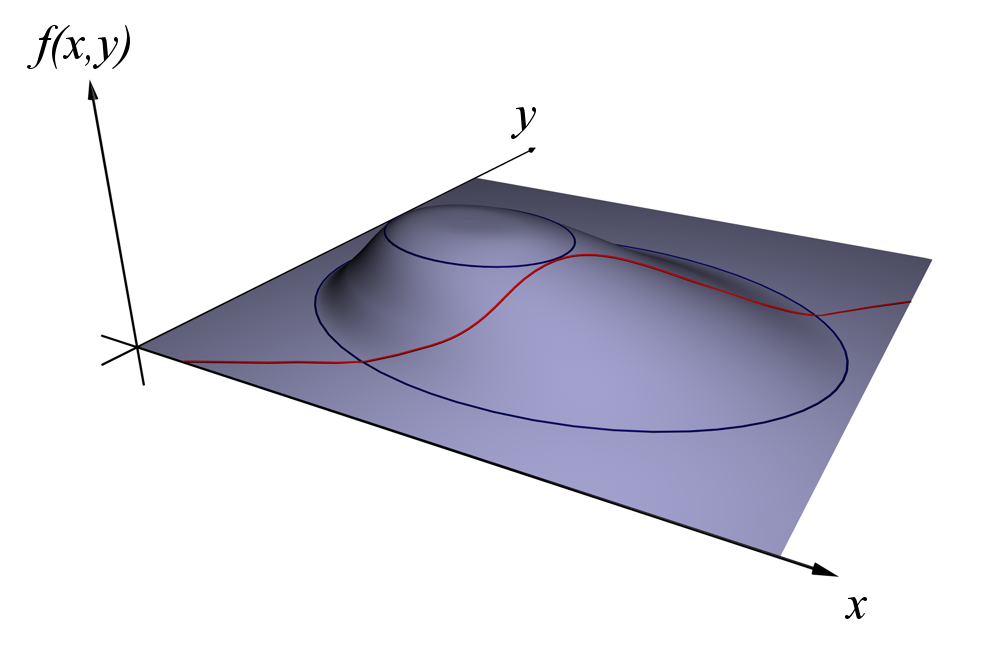
Geometrically:

• $\nabla f(\vec{a})$ is parallel to $\nabla g(\vec{a})$:

• $g(x)$ is tangential to a level set of $f$ at $\vec{a}$:
  • This is because the gradient vector of $f$ is always perpendicular to the contour.

Explanation §

(Assuming $g:{\mathbb{R}}^n\to \mathbb{R}$ is a scalar function, and we are finding the maximum.)

Lagrange multipliers work on some basic assumptions:

• The gradient vector points towards the direction of steepest ascent. That is, $\nabla f(\vec{x})$ points towards closest highest value of $f$ from $\vec{x}$ unless $\nabla f(\vec{x})=\vec{0}$
• The level set of a function is always perpendicular to its gradient vector.

Okay, let’s get started:

1. We know that the highest local extrema are when $\nabla f=\vec{0}$. However, it could be that these extrema do not satisfy the constraint function $g$.

2. One way of ensuring we always satisfy the $g$ constraint is to treat $g(\vec{x})=0$ as a level set. As we travel along the level curve of $g$, we need to find the point $\vec{x}$ that maximises the value of $f$.

3. As we travel along this level curve, one of three things can happen:

   • We could be travelling in a way such that we are cutting through the level sets of $f$. That is, we are travelling perpendicularly to these level sets.
   • We could be travelling in a way such that we are going along with some level set of $f$. That is, we are travelling parallelly to these level sets.
   • We could could be doing neither.

4. If we are travelling by cutting through level sets, then we are travelling parallel to the gradient vector of $f$ (see assumption), i.e. we are parallel to $\nabla f(\vec{x})$. These means we are going towards the extrema, but we haven’t found it.

   • If we are at some point $f(\vec{b})$ and are travelling along this way, then we know $\vec{b}$ cannot be an extrema because we can just go to a level set that is ‘higher’ or ‘lower’

5. If we travel parallel to the level set, then all the values $f(\vec{x})$ are the same, so even if one of these points is an extrema, they all become extrema.

6. Then what we need to do is to first travel as parallel to the gradient vector of $f$ as possible (to ensure most increase) then at some point we should be parallel to a level curve (so we know there is no higher point).

7. That is, our level curve of $\vec{g}$ should be tangential to a level set of $f$. Since by definition, a tangent touches a curve at exactly one point.

8. We can then use the second assumption. If we make $\nabla \vec{g}$ and $\nabla \vec{f}$ parallel at some point $\vec{a}$, then that makes $f$ and $g$ tangential at that point $\vec{a}$. The equation for parallel vectors results in:

$$\nabla f(\vec{a})=\lambda g(\vec{a})$$

We also add the restriction $g(\vec{a}) \neq \vec{0}$, because the zero vector is parallel to *every vector*, which doesn't really help us.

9. This also captures any local extrema of $f$ because if we set $\lambda =0$, we find these extrema.

Visualisation §

#todo

Theorems §

T1: Superposition of Lagrange Multipliers ^t1

Let $f,g_1,g_2$ be $C^1$ smooth functions. $f:{\mathbb{R}}^n\to \mathbb{R}$ is the objective function. Let the constraint functions be $g_1,g_2:{\mathbb{R}}^n\to {\mathbb{R}}^c$. If we have, for $g_1(\vec{x})=\vec{0}$ and $g_2(\vec{x})=\vec{0}$. Let $\vec{a}$ be a point $(a_1,\dots ,a_n)\in {\mathbb{R}}^n$. If we have:

• $\nabla g_1(\vec{a})$ and $\nabla g_2(\vec{a})$ are linear independent.
• $\nabla g_1(\vec{a})$ and $\nabla g_2(\vec{a})$ are both non-zero vectors ($\ne \vec{0}$).

Then:

$$\exists {\lambda }_1,{\lambda }_2\in \mathbb{R},\nabla f(\vec{a})={\lambda }_1\nabla g_1(\vec{a})+{\lambda }_2\nabla g_2(\vec{a})⟹\text{a is an extremum of f subject to the constraints g1,g2}$$

That is, if the gradient vector $\nabla f$ at the point $a$ can be written as the linear combination of the gradient vectors $\nabla g_1,\nabla g_2$ at the point $a$, then $a$ is an extremum etc. etc. This is known as the superposition of Lagrange multipliers and can be used to solve linear programs for multiple constraints.

Examples §

E1: Paraboloid constrained to an ellipse

Find the maximal and minimal values of $f$ (i.e. the extrema) subject to the constraint $g(x,y)=0$ where:

$$f(x,y)=x^2+y^{2}g(x,y)=\frac{x^2}{4}+y^2-1$$

Solution $g(x,y)=0$ defines a ellipse. We start by finding the gradient vectors for both $f$ and $g$:

Note that

$$\nabla f=\left(\frac{\partial f}{\partial x},\frac{\partial f}{\partial y}\right)=(2x,2y)\nabla g=\left(\frac{\partial g}{\partial x},\frac{\partial g}{\partial y}\right)=(\frac{x}{2},2y)$$

We use the Lagrange multipliers equation, combined with the restriction that $g(x,y)=0$

$$\nabla f=\lambda \nabla g\text{ and }\frac{x^2}{4}+y^2-1=0$$

Solving results in a system of equations:

$$\{\begin{array}{l}2x=\frac{\lambda x}{2}⟹\lambda =4\\ 2y=2\lambda y⟹\lambda =1\end{array}$$

#todo

E2: Volume-Area Optimisation

An open rectangular box needs to be constructed with a volume of $4{\text{m}}^3$. What dimensions should the box be to minimised the material used?

Solution surface area of the box. Also, an open rectangular box implies it is a cuboid without one face. Hence, we have volume and surface area given by:

Firstly, note minimising the material used is the same as minimising the

$$V(x,y,z)=xyzA(x,y,z)=2xy+2yz+2xz-xy=2z(x+y)-xy$$

We are minimising $f(x,y,z)=A(x,y,z)$ subject to the constraint function $g(x,y,z)=V(x,y,z)-4$. Let’s start with the gradient vectors:

$$\begin{array}{rl}\nabla f& =\left(\frac{\partial f}{\partial x},\frac{\partial f}{\partial y},\frac{\partial f}{\partial z}\right)=(y+2z,x+2z,2xy)\\ \nabla g& =\left(\frac{\partial g}{\partial x},\frac{\partial g}{\partial y},\frac{\partial g}{\partial z}\right)=(yz,xz,xy)\end{array}$$

We then use the Lagrange multipliers equation, combined with the equation $g(x,y,z)=0$:

$$\nabla f=\lambda \nabla g\text{ and }xyz-4=0$$

Solving the system of equations:

$$\{\begin{array}{l}y+2z=\lambda yz\\ x+2z=\lambda xz\\ 2x+2y=\lambda xy\\ xyz=4\end{array}$$

• We assume all the dimensions to be positive, $x,y,z>>0$
• We can express $z$ using $x,y$ in the 4th equation: $xyz=4⟹z=\frac{4}{xy}$. We assume that that we must maximise the box such that it is symmetrical in the x and y axis, (since the only ‘modification’ is that the box has an open z-face). Hence $z=\frac{4}{x^2}$ (assuming $x=y$)
• Combining equations (1) - (2): $(1)-(2):y-x=\lambda z(y-x)$
• Again, by symmetry we can modify equation 3: $4x=\lambda x^2⟹x\cdot (4-\lambda x)=0$. The solutions are $x=0$ or $x=\frac{4}{\lambda }$. But since $x>>0$, the only solution is $x=\frac{4}{\lambda }$
• Then, by symmetry, $y=\frac{4}{\lambda }$. And by equation (4): $z=\frac{4}{{\left(\frac{4}{\lambda }\right)}^2}=\frac{{\lambda }^2}{4}$
• Finally, we can use equation (2): $x+2z=\lambda xz⟹\frac{4}{\lambda }+\frac{{\lambda }^2}{2}={\lambda }^2⟹8={\lambda }^3$
• Hence $\lambda =2$

So our solution $(x,y,z)=(2,2,1)$

#todo composition of lagrange multipliers

Resources §

• https://www.youtube.com/watch?v=8mjcnxGMwFo