Gallery Of Functions

$x^2+y^2$ §

\usepackage{pgfplots}
\pgfplotsset{width=15cm,compat=1.16}
 \begin{document}
 
 \begin{tikzpicture}
 \begin{axis}[colormap/bluered]
 \addplot3[
 	mesh,
 	samples=30,
 	domain=-3:3
 ]
 {x^2 + y^2}; 
 \end{axis}
 \end{tikzpicture}
 \end{document}

$x^2+y^2$ subject to the constraint $\frac{x^2}{4}+y^2=1$ §

%% ```tikz \usepackage{pgfplots} \pgfplotsset{width=15cm,compat=1.16} \begin{document}

\begin{tikzpicture} \begin{axis}[colormap/bluered] \addplot3[ mesh, samples=30, domain=-3:3, axis equal ] {x^2 + y^2}; \addplot[domain=0:360,samples=200,blue,thick] ({2cos(x)},{sin(x)}); \addplot[domain=0:360,samples=200,blue,thick] ({4cos(x)},{2*sin(x)}); \end{axis} \end{tikzpicture} \end{document}

$x^2-y^2$ §

\usepackage{pgfplots}
\pgfplotsset{width=15cm,compat=1.16}
 \begin{document}
 
 \begin{tikzpicture}
 \begin{axis}[colormap/bluered]
 \addplot3[
 	mesh,
 	samples=30,
 	domain=-3:3
 ]
 {x^2 - y^2}; 
 \end{axis}
 \end{tikzpicture}
 \end{document}

$\frac{x^2}{x^2+y^2}$ §

\usepackage{pgfplots}
\pgfplotsset{width=20cm,compat=1.16}
 \begin{document}
 
 \begin{tikzpicture}
 \begin{axis}[colormap/bluered]
 \addplot3[
 	mesh,
 	samples=20,
 	domain=-3:3
 ]
 {x^2/(x^2 + y^2)};
 \end{axis}
 \end{tikzpicture}
 \end{document}

$\frac{xy}{x^2+y^2}$ §

\usepackage{pgfplots}
\pgfplotsset{width=20cm,compat=1.16}
 \begin{document}
 
 \begin{tikzpicture}
 \begin{axis}[colormap/bluered]
 \addplot3[
 	mesh,
 	samples=30,
 	domain=-3:3
 ]
 {(x*y)/(x^2 + y^2)};
 \end{axis}
 \end{tikzpicture}
 
 \end{document}

$\frac{x^2}{\sqrt{x^2+y^2}}$ §

\usepackage{pgfplots}
\pgfplotsset{width=20cm,compat=1.16}
 \begin{document}
 
 \begin{tikzpicture}
 \begin{axis}[colormap/bluered]
 \addplot3[
 	mesh,
 	samples=20,
 	domain=-3:3
 ]
 {x^2/sqrt(x^2 + y^2)};
 \end{axis}
 \end{tikzpicture}
 \end{document}

$xy-y-x+3$ §

 \usepackage{pgfplots}
\pgfplotsset{width=10cm,compat=1.16}
 \begin{document}
 \begin{tikzpicture}
\begin{axis}
 % Surface restricted to triangular domain
 \addplot3[
    surf,
    domain = 0:2,
    y domain = 0:4,
    restrict expr to domain={2*x+y}{0:4}
]
{ x*y - y - x + 3 };

 % Full mesh for reference
 \addplot3[
    mesh,
    domain = -2:2,
    y domain = -4:4,
]
{x*y - y - x + 3};

\end{axis}
\end{tikzpicture}
\end{document}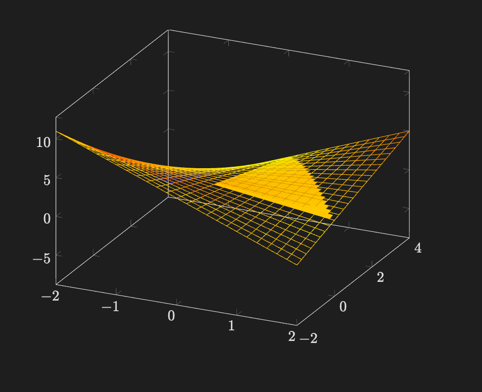

$(\cos (t),\sin (t),t)$ §

\usepackage{pgfplots}
\pgfplotsset{width=10cm,compat=1.16}
 \begin{document}
 \begin{tikzpicture}
\begin{axis}
[zmin = 0, zmax = 4*360, xmin = -2, xmax = 2, ymin=-2, ymax = 2]
 % Surface restricted to triangular domain
 \addplot3[
    mesh,
    samples = 50,
    variable = t,
    domain = 0:1440
]
({cos(t)}, {sin(t)}, {t});
\end{axis}
\end{tikzpicture}
\end{document}

Kinematic Path §

\usepackage{pgfplots}
\pgfplotsset{width=10cm,compat=1.16}
 \begin{document}
 \begin{tikzpicture}
\begin{axis}[view = {50}{-30}]
 % Surface restricted to triangular domain
 \addplot3[
    mesh,
    variable = t,
    domain = 0:10
]
({3*t+2}, {t^2 - 7}, {t - t^2});
\addplot3[
variable = s, domain = -5:10]
({2 + 3*s}, {-8 + 2*s}, {1 - s});
\end{axis}
\end{tikzpicture}
\end{document}

Parametric Cone §

With Normal Vector Field §

\usepackage{pgfplots}
\pgfplotsset{width=10cm,compat=1.16}

\begin{document}
\begin{tikzpicture}
\begin{axis}[zmin=0, zmax=6, view={30}{30}, axis equal]
    % Parametric cone
    \addplot3[
        mesh,
        domain=0:2*pi,
        domain y=0:6,
        samples=40
    ]
    ({y*cos(deg(x))}, {y*sin(deg(x))}, {y});

    % Normal vectors
    \addplot3[
        cyan,
        quiver={
            u={-x},  % x-component of normal
            v={-y},  % y-component of normal
            w={z},             % z-component of normal
            scale arrows=0.1
        },
        -stealth,
        samples=10,
        domain=0:2*pi,
        domain y=0.5:6 % avoid y=0 at tip
    ]
    ({y*cos(deg(x))}, {y*sin(deg(x))}, {y});

\end{axis}
\end{tikzpicture}
\end{document}

With Tangent Plane §

\usepackage{pgfplots}
\pgfplotsset{width=10cm,compat=1.16}

\begin{document}
\begin{tikzpicture}
\begin{axis}[zmin=0, zmax=6, view={30}{30}, axis equal]
    % Parametric cone
    \addplot3[
        mesh,
        domain=0:2*pi,
        domain y=0:6,
    ]
    ({y*cos(deg(x))}, {y*sin(deg(x))}, {y});

    \addplot3[
        mesh,
        domain=-6:6,
        domain y=-6:6,
    ]
    {(1/sqrt(2)) * (x + y)};

\end{axis}
\end{tikzpicture}
\end{document}