Just like how Gauss’ Law makes it easy to solve complex charge distributions, Ampère’s Law simplifies calculating magnetic fields for current flowing through complex shapes.
#todo Applications!!
Definition
Assume we define a closed loop around some current carrying object. Then:
Ampère's Law
\oint \vec{B} \cdot d\vec{l} = \mu_{0} I_{enclosed}
>[!terms]- >* $\vec{B}$ = [Magnetic Field](Magnetic%20Field.md) (in $T$) >* $\vec{l}$ = Path vector of the loop. $d\vec{l}$ returns an infinitesimally small section of said path. >* $\mu_{0}$ = Permeability of free space >* $I_{enclosed}$ = [Current](Current.md) enclosed inside the loop. >* $\oint$ = Line integral
Unfinished...
This law is very useful in obtaining the relationship between current and magnetic fields, but there is another way a magnetic field can be created - through a changing Electric Field! The addition is shown in the revised Ampère-Maxwell Law.
Derivation
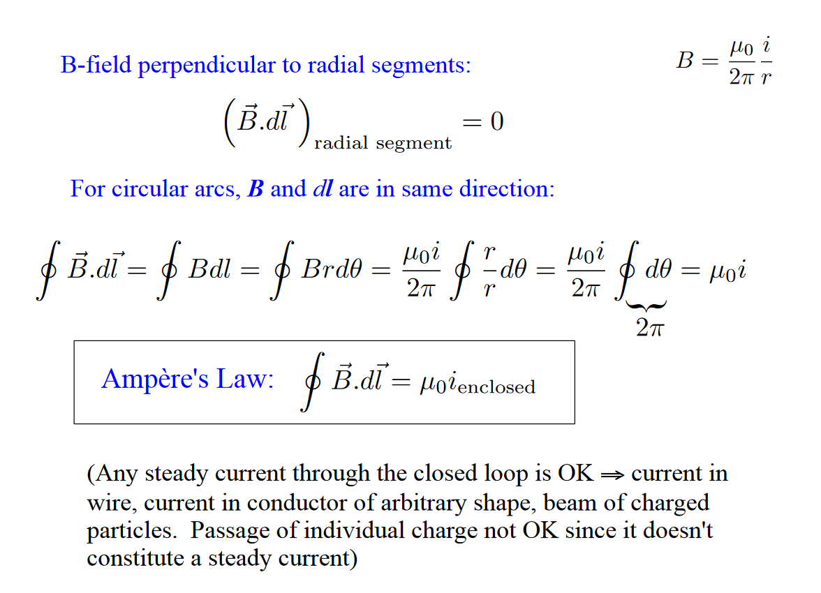
Ampere’s Law is derived from the Biot-Savart Law, when applied through a Infinite Line of Current. The formula is given by:
Observe what happens if we decide to take a circular loop around the wire:
The circumference of this loop is given by: . And if we define this loop to be made up of infinite then:
If we now look at the magnetic field in this loop:
Now let’s look at a more complex loop:
This loop consists of areas where (in red) and (in green):